Testing wave behavior across a phase transition

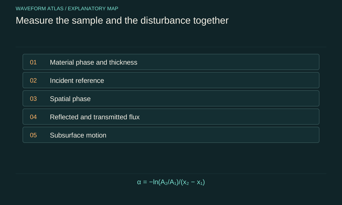
Choose a comparison that isolates the transition

An experiment across freezing compares systems whose properties may change simultaneously. Temperature, solid fraction, thickness, surface roughness and mechanical contact can all vary. A smaller wave signal after cooling therefore does not identify a single cause. Begin with a specific question, such as whether the measured dispersion changes when a continuous cover forms, or whether an incident pulse loses more energy to dissipation after a specified structural change.

The question determines the required observables. A dispersion measurement needs frequency and spatial phase. An attenuation measurement needs calibrated amplitude at several positions and control of reflections. An energy-loss claim needs a flux account and, where feasible, independent information about dissipative channels. A picture can document morphology, but it cannot substitute for every one of these measurements.

Record the material state rather than temperature alone

Temperature indicates one aspect of the thermal condition. During phase coexistence, latent heat can change the solid fraction while the temperature remains near the transition value. Conversely, a temperature gradient can leave different parts of the sample in different states. Record where temperatures are measured and how those locations relate to the wave path.

Characterize thickness, coverage, connectivity and visible defects of the solid region. A continuous sheet and a collection of floating crystals can have very different responses at the same nominal temperature. Thermal history also matters: cooling and warming runs can produce different structures. Treat those differences as physical variables to document, not merely as inconvenient scatter in an otherwise identical dataset.

Measure the incident field independently

A source driven with the same voltage need not deliver the same mechanical wave after the medium changes. Its loading, coupling and resonance can shift. Place a reference measurement where the incoming field can be estimated, and separate it from reflected contributions where possible. This establishes what actually reaches the region under study.

For a pulse, record its temporal shape and spectrum. For a nearly monochromatic drive, record amplitude, frequency stability and harmonic content. A change in the source spectrum can mimic material dispersion or frequency-dependent attenuation. Normalizing the output by the commanded drive alone is therefore weaker than normalizing it by a calibrated measurement of the incident disturbance.

Spatial phase reveals a changed propagation law

Use several positions along the propagation direction to estimate phase accumulation. For a single dominant mode, phase differences can constrain wavenumber at each frequency. Combining wavenumber and frequency gives a measured dispersion relation. Phase unwrapping and sensor separation must be chosen carefully because differences larger than a cycle can create ambiguity.

If more than one mode is present, a single phase slope can be misleading. Reflected waves, bending modes and local edge motion may overlap. Spatially resolved measurements or a model that includes several components can separate them. The objective is not merely a smooth fitted curve, but a mode assignment supported by propagation direction, polarization or displacement structure and the relevant boundary conditions.

Attenuation requires a model of geometry

In a simple uniform one-dimensional model, an amplitude may decay as A(x) = A₀ exp(−αx). The corresponding intensity contribution then scales as exp(−2αx) when the mode normalization is unchanged. A fitted intensity attenuation coefficient is therefore not numerically interchangeable with an amplitude attenuation coefficient. State the convention and units.

Geometrical spreading can reduce amplitude without dissipation. A wave radiating outward spreads energy over a growing area, while a guided wave may not. Reflection from boundaries can create standing-wave maxima and minima that corrupt a single exponential fit. Before interpreting α as a material loss parameter, account for the geometry and isolate the traveling component to which the model applies.

A simple ratio illustrates uncertainty

Suppose two calibrated sensors one meter apart measure amplitudes of 1.00 and 0.80 in arbitrary displacement units for the same traveling mode. The exponential model gives α = −ln(0.80)/1 m, approximately 0.223 per meter. This is an illustrative calculation. If each amplitude has independent relative uncertainty of two percent, the ratio has roughly 2.83 percent relative uncertainty, giving an approximate α uncertainty of 0.028 per meter.

Shared calibration errors can partly cancel in the ratio, while sensor-specific errors do not. If reflections produce an additional unknown phase-dependent contribution, the simple uncertainty estimate is incomplete. Repeating the measurement at several separations and swapping sensors helps identify systematic effects. A precise numerical fit is not a substitute for a valid forward model.

Look beneath a visually quiet surface

An ice cover can alter the relationship between visible surface displacement and motion below it. Measurements of pressure or fluid velocity can reveal energy that a surface camera misses. Motion of the cover itself can identify bending or rigid-body response. The grease-ice experiment by Rabault and colleagues is a relevant source example because it combined elevation measurements with particle image velocimetry in a tank.

That verified source supports the value of complementary observables, not a universal numerical attenuation law for all frozen media. A new experiment should choose instruments appropriate to its own opacity, geometry and length scales. If particles or markers are used to infer flow, their ability to follow the relevant motion must be assessed. Every measurement method has a response function and a range over which it is trustworthy.

Separate the background heat flow

Freezing requires substantial heat transport, often much larger than the heating associated with a weak wave. A thermal signal during solidification cannot automatically be assigned to wave dissipation. Compare driven and undriven conditions with closely matched thermal histories, and determine whether the expected wave contribution is resolvable above the changing background.

Likewise, a change in attenuation can reflect structural evolution during the measurement. Record time since preparation and front position, and repeat at comparable states rather than merely comparable clock times. If the sample evolves too rapidly for a steady-state measurement, use a time-dependent analysis. Calling the sample stationary while its material properties drift can create artificial frequency dependence and apparent nonlinearity.

Use controls that target competing mechanisms

To distinguish reflection from loss, measure upstream and downstream signals. To distinguish a mode conversion from simple attenuation, inspect displacement patterns and spectra. To distinguish an optical imaging artifact from mechanical suppression, compare with an independent sensor. To test whether the transition itself matters, compare nearby conditions with different solid fractions while controlling the incident field as closely as possible.

A control should remove or alter one explanatory ingredient without silently changing several others. Perfect isolation is often impossible, so document the remaining couplings and uncertainty. The most useful experiment is not necessarily the one with the most instruments. It is the one whose measurements constrain the specific alternatives that would otherwise produce the same apparent disappearance of a ripple.

Report a bounded conclusion

A strong result might establish that a measured dispersion curve becomes consistent with a thin-plate model over a stated frequency band, or that a traveling-wave amplitude decays faster after a defined structural change. It should state the model, bandwidth, material condition and uncertainty. If unmeasured channels remain, describe the missing energy as unaccounted for rather than declaring it absorbed.

The phase transition can produce several effects at once: new restoring forces, altered inertia, scattering, dissipation and changed optical visibility. A complete account keeps those channels separate long enough to test them, then combines the supported contributions into one physical explanation. That approach turns freezing from a visual label into a reproducible study of how material state controls wave propagation.

Repeat the transition, not just the acquisition

Many repeated camera frames from one freezing event quantify measurement repeatability within that event. They do not establish reproducibility across independently prepared samples. If grain structure, cracks or cover connectivity vary between transitions, those variations can dominate the physical response even when each individual trace is measured precisely.

Separate within-run uncertainty from between-run variability. Repeat the preparation when feasible, document the resulting material state and compare wave observables at matched conditions. A hierarchical description of the data can distinguish detector noise from sample-to-sample differences. Averaging all traces into one smooth curve without preserving that distinction can produce unjustifiably narrow error bars.

Heating and cooling cycles also test hysteresis. Different responses at the same temperature can be legitimate consequences of different structures rather than failed measurements. If hysteresis is observed, the state description must include the preparation path. The resulting conclusion may be less universal, but it is more physically informative: it identifies the material features that need control before a propagation law can be transferred to another sample or operating condition.

Finally, retain the raw synchronized records and the exact calibration version used for analysis. A processed amplitude map can hide phase, timing and baseline choices that later become important. Reanalysis with a revised material model is much more informative when the original sensor signals, sample images and front trajectories remain linked to the same experimental run.

Go to the original work.

These links identify the sources behind specific claims. Verification scope varies by source and is stated below.

1. 1 / University teachingOpenStax University Physics Volume 2: Phase Changes ↗

   OpenStax University Physics Volume 2: Phase Changes. https://openstax.org/books/university-physics-volume-2/pages/1-5-phase-changes

   Phase coexistence, latent heat and the distinction between temperature and phase.

   Verification scope: Open textbook section inspected; no claim that cooling always produces a solid.

2. 2 / Primary theoryWaves due to a steadily moving source on a floating ice plate ↗

   J. W. Davys; R. J. Hosking; A. D. Sneyd. Journal of Fluid Mechanics 158, 269–287 (1985).

   DOI: 10.1017/S0022112085002646

   Flexural–gravity wave propagation in an idealized floating ice plate.

   Verification scope: Publisher or author-institution abstract and bibliographic record inspected; full paper not audited.

3. 3 / Primary experimentExperiments on wave propagation in grease ice: combined wave gauges and particle image velocimetry measurements ↗

   Jean Rabault; Graig Sutherland; Atle Jensen; Kai H. Christensen; Aleksey Marchenko. Journal of Fluid Mechanics 864, 876–898 (2019).

   DOI: 10.1017/jfm.2019.16

   Joint surface and flow measurements in a wave–grease-ice experiment.

   Verification scope: Publisher or author-institution abstract and bibliographic record inspected; full paper not audited.

4. 4 / University teachingMIT Physics III: Vibrations and Waves ↗

   Yen-Jie Lee. MIT Physics III: Vibrations and Waves. 2016.

   Wave equations, interfaces, optics and propagation in media.

   Verification scope: MIT course outline inspected; article derivations are independent textbook-level explanations.