When instruments make waves look flat

Model the measurement chain

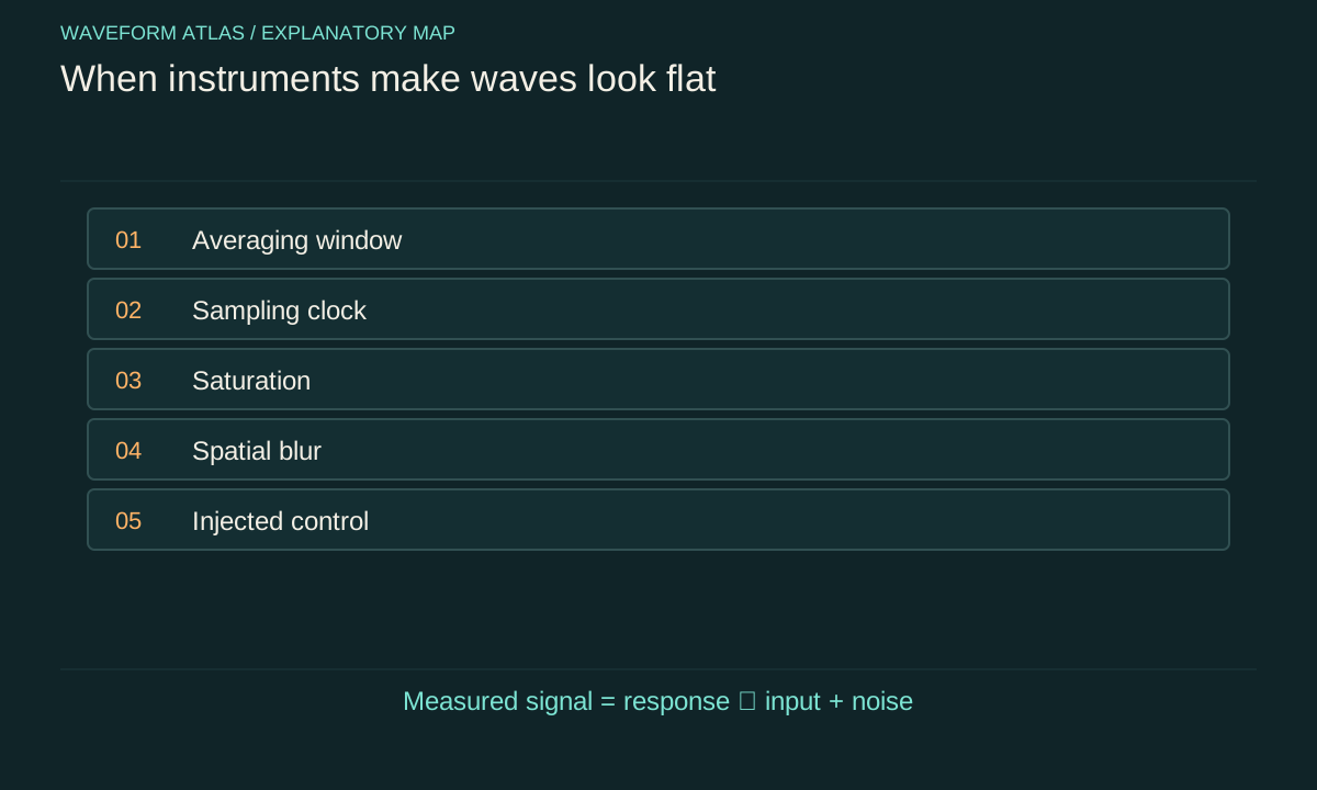
A detector does not deliver the field itself. It converts a physical input into an electrical or digital output through a response that can include filtering, integration, amplification and sampling. A useful linear model writes the recorded signal as the true signal convolved with an instrument response, plus noise. Nonlinearities such as saturation require additional terms or a different description. The model identifies what information the instrument can preserve.

A flat record may therefore originate in the source, the detector or the processing. Begin by naming the measured quantity and units. A camera often measures an integrated intensity, a microphone measures pressure through a frequency-dependent sensitivity, and a phase-sensitive receiver measures a selected quadrature. These outputs cannot be interpreted interchangeably. The physical claim should follow the quantity actually measured, not the generic label wave signal.

Integration can cancel a signed oscillation

An instrument that averages a signed sinusoid over many cycles can return a value close to zero. For a rectangular integration window of duration T, the response to a sinusoid depends on the factor sin(ωT/2)/(ωT/2), together with its phase. At certain window lengths the average vanishes exactly in the ideal model. The underlying oscillation remains present throughout the interval.

Change the integration duration and compare the results. If the apparent suppression tracks the expected averaging response, the evidence points to the measurement window. An intensity detector behaves differently because it averages a quadratic quantity that generally remains positive. Record whether the device averages a field, its square or a processed envelope. A zero signed average cannot be substituted for a zero mean-square measurement.

For a window centred at t₀, direct integration gives (1/T)∫[t₀−T/2,t₀+T/2] A cos(ωt+φ)dt=A cos(ωt₀+φ) sin(ωT/2)/(ωT/2). This is the article’s rectangular-window derivation, separate from the sampling theorem.

Sampling can freeze a moving waveform

A sinusoid sampled exactly once per period at the same phase produces identical samples. It can appear as a constant line even though it oscillates between samples. Sampling at twice the frequency is not a universal cure, because phase alignment and finite bandwidth still matter; practical reconstruction requires an adequate sampling rate and suitable antialias filtering for the signal band. Out-of-band components can otherwise masquerade as lower-frequency structure.

Repeat a suspected null measurement with a changed sampling rate or an independently timed instrument. A physical stationary signal should not acquire an apparent oscillation solely because the digital clock changed, whereas an aliased one often will. Preserve timestamps and any synchronization settings. A plot labelled only by sample index can conceal clock errors, dropped frames or irregular acquisition intervals that matter when interpreting wave dynamics.

Bandwidth determines what reaches the output

A detector with a slow response attenuates rapid changes. A high-pass stage can suppress a steady or slowly varying component. Cascaded amplifiers, cables and filters contribute to the total response. The useful bandwidth is therefore a property of the whole chain, not merely the sensor's advertised specification. Measure or verify that response under the operating conditions used for the experiment.

Inject a known test signal at several frequencies spanning the relevant range. Check amplitude and phase, since phase distortion can affect cancellation or inferred propagation delay. If the experiment changes the wave spectrum, a detector calibrated at only one frequency may report a false amplitude change. An observed reduction could mean the signal moved into a less sensitive part of the response rather than losing energy.

Saturation creates artificial plateaus

When a camera pixel or amplifier reaches its maximum output, further input no longer produces a proportional change. A peaked beam can then acquire a flat central region in the recorded image. The clipped profile is an instrument limit, not evidence that the physical intensity became uniform. Saturation can also generate harmonics and distort timing in an otherwise simple waveform.

Reduce the input through a calibrated attenuation or adjust the gain, then compare rescaled measurements in the linear range. A genuine plateau should retain its shape within uncertainty; a clipped one often reveals the hidden peak. Inspect raw values for repeated maxima and check whether the software automatically changes exposure. Automatic adjustments can make before-and-after images look comparable while concealing a large change in incident power.

Spatial averaging hides fine structure

A finite pixel or sensor aperture averages over a region. If alternating bright and dark features are much smaller than that region, the measured image can appear uniform. Optical blur adds another spatial filter. A flat image therefore establishes uniformity only after the instrument's spatial response has been applied. It does not exclude structure at scales the detector cannot resolve.

Measure a known edge, point or pattern to estimate resolution where appropriate. When comparing with theory, convolve the predicted distribution with that response before evaluating agreement. Deconvolution can help infer finer structure, but it amplifies noise and depends on assumptions. Present reconstructed and raw measurements separately, and avoid interpreting a smooth regularized reconstruction as direct evidence that the underlying field was smooth.

Processing can subtract the sought signal

Background subtraction, detrending, normalization and smoothing are useful operations when their purposes are explicit. They can also remove real physical components. Subtracting the mean guarantees that the processed record has zero mean, so that property cannot then be offered as an independent discovery. Normalizing each frame to its own maximum can conceal changing amplitude or power. A strong smoothing filter can erase transient peaks.

Keep the original data and document the processing sequence. Apply the same procedure to synthetic signals with known properties and to control measurements. If a method cannot recover an injected component similar to the proposed effect, its null result is not decisive. Define analysis choices before inspecting the final comparison when possible, especially if multiple filter settings could produce a visually satisfying flat trace.

Noise establishes a detection limit

A reading consistent with zero is usually a statement about uncertainty. Estimate detector noise and background under matched conditions, then determine what signal sizes the experiment could reliably distinguish. The standard error of an average decreases with sample count only according to the independence and stability of those samples. Correlations, drift and systematic offsets can prevent the simple square-root improvement expected for independent noise.

A practical report gives an upper bound on the measured amplitude or variance over a stated bandwidth and confidence procedure. It should also identify systematic uncertainty in calibration and subtraction. A bound is not a proof of exact mathematical zero. Conversely, a noisy trace does not automatically establish a physical fluctuation source; the instrument can contribute noise that must be separated from the field under study.

Reference drift can erase ensemble coherence

Phase-sensitive measurements rely on a reference whose relation to the source is known. If that reference drifts between trials, averaging can suppress the measured coherent component. Individual trials may still contain strong oscillations. Record a reference channel or estimate phase trial by trial where the protocol permits it. Compare unaligned and phase-aligned ensembles to determine how much apparent flattening comes from reference uncertainty.

The correction itself must be justified. Aligning trials using the same noisy signal can introduce bias, especially near the detection threshold. Test the procedure on controls and report its uncertainty. A recovered average supports a claim about correlations with the available reference; it does not imply arbitrary recovery after every possible environment interaction. The relevant question is which records and transformations the experiment actually provides.

A minimal diagnostic sequence

First inspect raw samples and acquisition settings. Next vary gain, exposure, sampling rate and bandwidth one at a time while preserving a calibrated input reference. Then inject a known signal and verify that the full analysis recovers it. Finally compare an independent detector or observable when the physical interpretation requires more than one quantity. Each step targets a different way the measurement chain can hide a wave.

The final conclusion should separate observed output from inferred input. For example, a calibrated pressure signal may be below a stated threshold over a defined band, while unmeasured frequencies remain unconstrained. Or a plateau may persist across linear exposure settings and known spatial resolution, supporting true intensity shaping. This discipline turns a visually flat graph into a reproducible measurement and makes clear which competing explanations the available controls have eliminated.

Suppose a detector samples a 50-hertz sinusoid at 50 samples per second. With a fixed phase relation, every sample has the same value and the plotted sequence is constant. If the sampling rate changes to 51 samples per second, the same physical sinusoid can appear as a one-hertz aliased oscillation in the samples. Nothing in the source needs to change.

This example assumes ideal regular sampling and no antialias filter that removes the 50-hertz component. A real acquisition chain may reject the signal before digitization, producing a different result. Record both the analog response and the digital sampling rate. A software setting alone cannot establish that an unrecorded high-frequency field was physically absent, and resampling an already aliased record cannot restore information that the original acquisition discarded.

Go to the original work.

These links identify the sources behind specific claims. Verification scope varies by source and is stated below.

1. 1 / University teachingMIT Quantum Physics I, Defining uncertainty ↗

   Variance is the second moment minus the square of the first moment.

   Verification scope: Official lecture transcript inspected.

2. 2 / University teachingMIT 6.300 Signal Processing: Sampling and Aliasing ↗

   MIT 6.300 Signal Processing, Week 3 Lecture A: Sampling and Aliasing (Fall 2025).

   Sampling ambiguities, Nyquist limit and antialias filtering; finite rectangular-window response is derived explicitly in the article.

   Verification scope: Lecture handout sampling/aliasing pages inspected directly.